Monte Carlo Simulation of your own Stata command with Mata-generated data.
Discrete Choice Models Mata Stata mlThis the final step of a series of earlier post where I dealed with the combination of a Mata evaluators within ado files that uses ml to fit Maximum Likelihood Estimations. Here a single dofile is used but it relies in what we have done in my previous post when we built up MyClogit command.
The only file needed is the following, and it can be downloaded by clicking on it.
MyMonteCarlo program
The first step is to define a program that we will then call using -simulate-. This follows the same structure of our past programs. Also in the middle the mata function data_gen() (listed below)is invoked, to generate the chosen alternatives. Finally it just invoke again MyClogit to fit the model.
capture program drop MyMonteCarlo
program define MyMonteCarlo, rclass
    version 12
    drop _all
    set obs 1000
    gen id = _n
    local n_choices =3
    expand `n_choices'
    bys id : gen alternative = _n


    // Regressors
    gen x1 =  runiform(-2,2)
    gen x2 =  runiform(-2,2)
    matrix betas_st = (0.5,2)

    // Calling generating data
    mata: data_gen()

    // Fitting the model
    MyClogit choice  x* , group(id)

end
Data Generation
We used a void matrix in Mata to create the data. This Mata function is invoked by MyMonteCarlo. This way to similate the data was highly inspired by this post in Statalist.
mata:
void data_gen()
{
        betas =st_matrix("betas_st")

        st_view(X = ., ., "x*")
        st_view(panvar = ., ., "id")
        paninfo = panelsetup(panvar, 1)
        npanels = panelstats(paninfo)[1]


        for(n=1; n <= npanels; ++n) {

            x_n = panelsubmatrix(X, n, paninfo)
            // Linear utility
            util_n =betas :* x_n
            util_sum =rowsum(util_n)
            U_exp = exp(util_sum)
            // Probability of each alternative
            p_i =     U_exp :/ colsum(U_exp)

            cum_p_i =runningsum(p_i)
            rand_draws = J(rows(x_n),1,uniform(1,1))
            pbb_balance = rand_draws:<cum_p_i
            cum_pbb_balance = runningsum(pbb_balance)
            choice_n = (cum_pbb_balance:== J(rows(x_n),1,1))


            if (n==1)     Y =choice_n
            else Y=Y \ choice_n

         }

        resindex = st_addvar("byte","choice")
        st_store((1,rows(Y)),resindex,Y)
}
end
Monte Carlo Simulation
To perform the simulations we used -simulate- which is a fairly simple way to run reapead times a model while saving relevant results. In this way we invoke MyMonteCarlo program and we run it 1000 times with a seed(157) for replicability.
simulate _b _se , reps(1000) seed(157) : MyMonteCarlo
command: MyMonteCarlo
Simulations (1000)
----+--- 1 ---+--- 2 ---+--- 3 ---+--- 4 ---+--- 5
.................................................. 50
.................................................. 100
.................................................. 150
.................................................. 200
.................................................. 250
.................................................. 300
.................................................. 350
.................................................. 400
.................................................. 450
.................................................. 500
.................................................. 550
.................................................. 600
.................................................. 650
.................................................. 700
.................................................. 750
.................................................. 800
.................................................. 850
.................................................. 900
.................................................. 950
.................................................. 1000
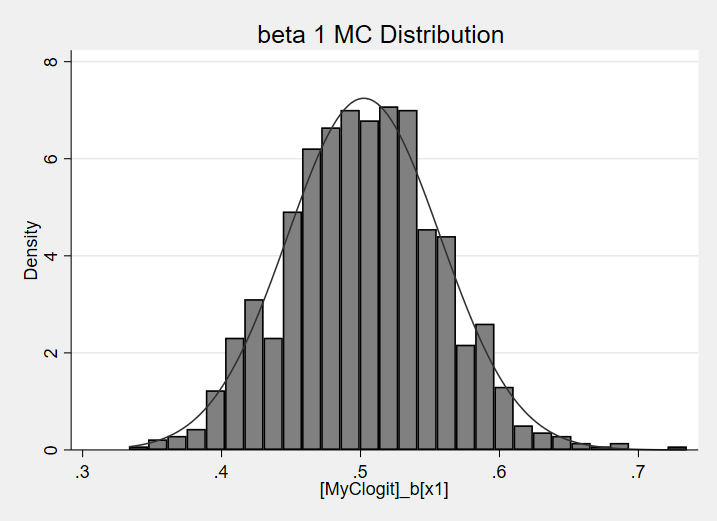
hist MyClogit_b_x1, scheme( sj ) den norm title("beta 1 MC Distribution ")
graph export b1.png ,replace
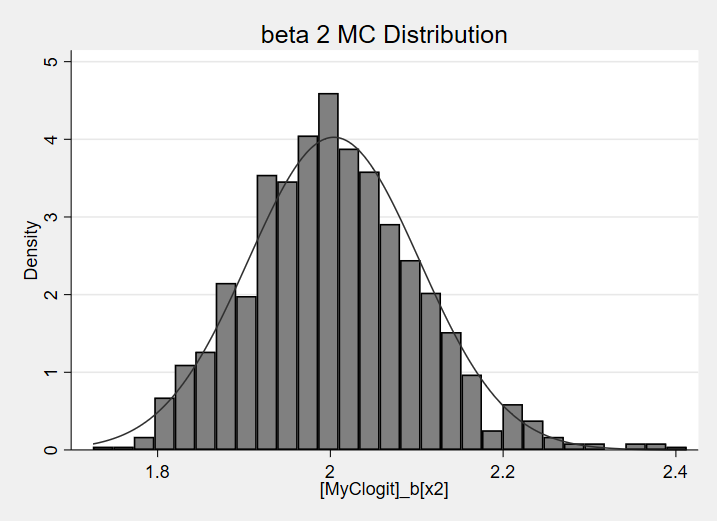
hist MyClogit_b_x2, scheme( sj ) den norm title("beta 2 MC Distribution")
graph export b2.png ,replace
Histograms of the results
References
Gould, W., Pitblado, J., & Sribney, W. (2006).. Maximum likelihood estimation with Stata. Stata press.
https://blog.stata.com/2015/10/06/monte-carlo-simulations-using-stata/
https://stats.idre.ucla.edu/stata/faq/monte-carlo-power-simulation-of-a-multilevel-model/